Let’s
Student Work
View More Student Work
this text will change
Become a Technical Artist
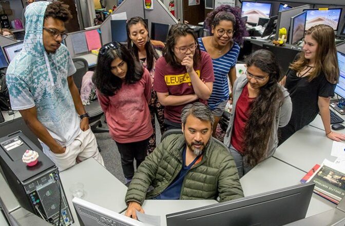
Where Art and Science Merge
We train technical artists to work on the collaborative teams necessary to make modern visualizations. Our programs produce leaders in the fields where art and science merge. We engage with the Aggie network and professional connections to give students professional exposure while earning their degree.
By the Numbers
Animation Career Review consistently ranks Texas A&M as a top school for animation, game design and graphic design.
#8
best public school in the nation for game design (2023)
#2
best public school in the nation for animation (2023)
#4
best school in in the nation for augmented/virtual reality (2022)